20.3 Analyse data
Data analysis is best described as looking at information carefully and making a decision. We can calculate the measures of central tendency, the measure of dispersion and interpret what the graphic representation of the data tells us. All these tools help us to understand and analyse the data and to identify any trends or patterns in the data.
Worked Example 20.3: Analysing data from a histogram
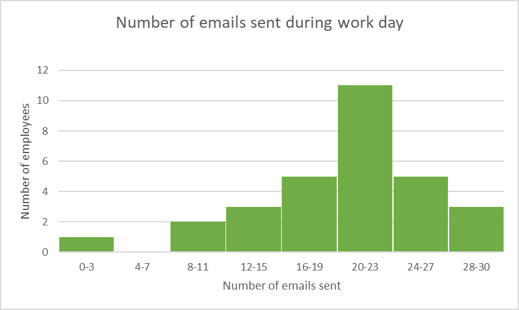
The graph below shows the number of emails sent per employee during a work day. Use the information to answer the questions.
- How many employees sent more than \(11\) emails?
- How many employees does the data in the graph represent?
- What percentage of employees sent less than \(12\) emails?
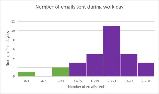
Determine how many employees sent more than \(11\) emails.
We can find the number of employees that sent more than \(11\) emails that day by adding up the heights of the five bins shown in purple below. We read the height of each bin using the scale on the vertical axis.
Number of employees that sent more than \(11\) emails \(=3 + 5 + 11 + 5 + 3 = 27\).
Find the number of employees represented in the data.
We can find the total number of employees by adding up the heights of all the bins.
Total number of employees \(= 1 + 2 + 3 + 5 + 11 + 5 + 3 = 30\).
Calculate the percentage of employees that sent less than \(12\) emails.
We can find the number of employees that sent less than \(12\) emails that day by adding up the heights of the two bins shown in blue below.
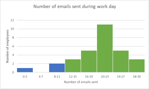
Number of employees that sent less than \(12\) emails \(=1 + 2 = 3\).
Percentage of employees that sent less than \(12\) emails:
\[\begin{align} &= \frac{\text{Number of employees that sent less than 12 emails}}{\text{Total number of employees}} \\ &= \frac{3}{30} \\ &= 10 \% \end{align}\]Worked Example 20.4: Analysing the effects of outliers on the mean and median of a data set
The heights (in centimetres) of \(10\) learners are measured to obtain the following data set:
\[150;172;153;156;146;157;157;143;168;157\]- Calculate the mean and median of the heights of the learners.
- One more learner needs to be included in the data set. This learner is very tall, with a measurement of \(181 \text{ cm}\). Calculate the mean and median of the heights of the \(11\) learners.
- How does the outlier (also called an extreme value) affect the values of the mean and median?
Determine the mean height of the \(10\) learners.
To calculate the mean value, we add up the heights of the learners and divide by the number of learners:
\[\begin{align} \text{Mean} &= \frac{150+172+153+156+146+157+157+143+168+157}{10} \\ &= \frac{1\ 559}{10} \\ &= \text{155,9} \text{ cm} \end{align}\]Find the median height of the \(10\) learners.
First we need to order the data set:
\[143;146;150;153;156;157;157;157;168;172\]There are \(10\) values in the data set. Since there is an even number of values, the median will be between the fifth and sixth value of the ordered data set:
\[\begin{align} \text{Median} &= \frac{156 + 157}{2} \\ &= \frac{313}{2} \\ &= \text{156,5} \text{ cm} \end{align}\]Determine the mean height of the \(11\) learners.
Now we include the height of the eleventh learner in the data set.
\[\begin{align} \text{Mean} &= \frac{150+172+153+156+146+157+157+143+168+157+181}{11} \\ &= \frac{1\ 740}{11} \\ &= \text{158,2} \text{ cm} \end{align}\]Find the median height of the \(11\) learners.
Include the data value to the ordered data set:
\[143;146;150;153;156;157;157;157;168;172; 181\]There are \(11\) values in the data set, so the median will be the sixth value of the ordered data set:
\[\text{Median} = 157 \text{ cm}\]Compare the different values for the mean and median.
From this we see that the average height changed by \(\text{158,2} − 155,9 = 2,3 \text{ cm}\) when we introduced the outlier value (the tall person) to the data set.
The median changed by \(\text{157} - \text{156,5} = \text{0,5} \text{ cm}\) when we included the outlier value in the data set.
In general, the median is less affected than the mean by the addition of outliers to a data set.